Cell Counting in Microscopy Images — U-Net & Attention U-Net
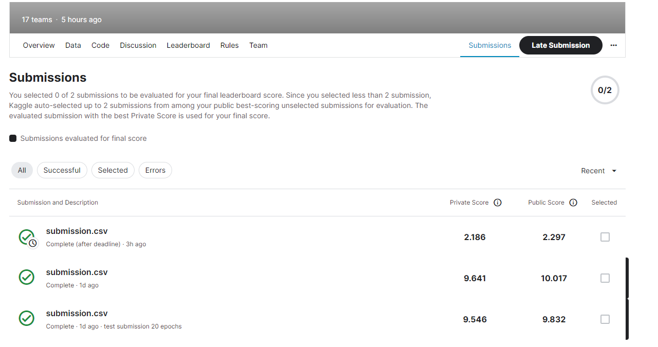
A deep learning pipeline for automated cell counting in fluorescence microscopy images. Trained a U-Net to predict binary segmentation masks of cell regions, then counted cells via connected-component labeling. Achieved a MAE of 2.186 on the Kaggle private leaderboard, improving from an initial score of ~10 through architectural changes, data augmentation, and loss function engineering.
Later revisited and expanded with an Attention U-Net variant (learned spatial focus on cell regions), Residual U-Net, multiple specialized loss functions (Dice, Focal, Tversky), elastic deformation augmentation following the original U-Net paper, and morphological post-processing with watershed segmentation for separating touching cells.
Competition Results
| Model | Augmentation | Loss | MAE (Private) |
|---|---|---|---|
| U-Net (32-base) | None | BCE | 9.57 |
| U-Net (64-base) | Flips + Rotation | BCE + Dice | 2.186 |
U-Net Architecture
Input (1×128×128 grayscale)
  ├― Encoder 1: 1 → 64     ――――――――――――――――――――――――― Skip ――┐
  ├― Encoder 2: 64 → 128   ――――――――――――――― Skip ――┐  │
  ├― Encoder 3: 128 → 256  ――――――― Skip ――┐  │  │
  ├― Encoder 4: 256 → 512  ― Skip ―┐  │  │  │
  ├― Bottleneck: 512 → 1024        │  │  │  │
  ├― Decoder 4: 1024 → 512 + cat ――└  │  │  │
  ├― Decoder 3: 512 → 256  + cat ――――└  │  │
  ├― Decoder 2: 256 → 128  + cat ――――――└  │
  ├― Decoder 1: 128 → 64   + cat ――――――――└
  └― 1×1 Conv → Output (1×128×128)

Each block: (Conv3×3 → BatchNorm → ReLU) × 2
Key Features
- Three model variants — Standard U-Net, Attention U-Net with learned spatial focus gates (Oktay et al. 2018), and Residual U-Net with identity shortcuts for better gradient flow
- Five loss functions — BCE, Dice, combined BCE+Dice, Focal Loss for class imbalance, and Tversky Loss for asymmetric FP/FN penalization to reduce missed cells
- U-Net paper augmentation — Elastic deformation with smoothed random displacement fields, plus random flips, rotations, Gaussian noise, and brightness/contrast adjustment
- Watershed post-processing — Morphological cleanup (opening/closing) followed by distance-transform watershed to separate touching cells
- Connected-component cell counting — Binary segmentation mask → connected components → area filtering → final cell count
- YAML-based experiment configs — Configurable hyperparameters, model selection, and loss functions via config files for reproducible experiments
Design Decisions
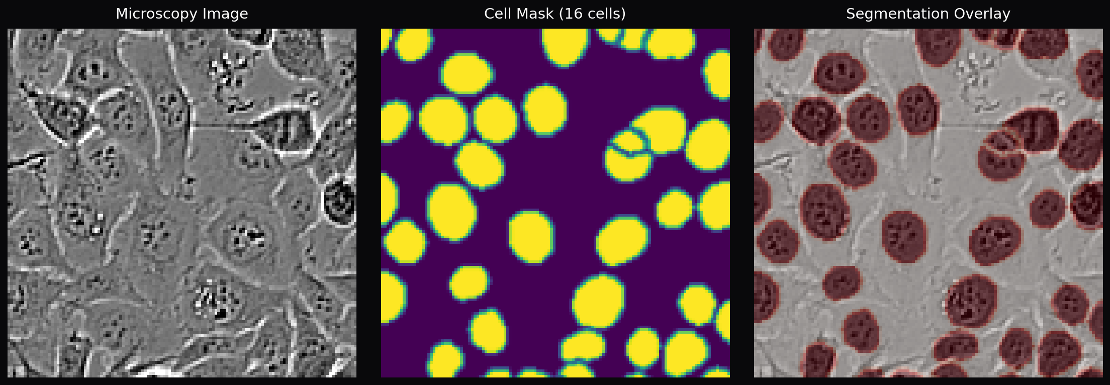
- Segmentation over regression — Rather than directly regressing cell counts, we segment individual cells and count via connected components. This provides interpretable intermediate results and enables visualization of where the model detects cells
- BCE+Dice combined loss — Pure BCE provides pixel-level gradients but ignores global overlap; pure Dice optimizes overlap but has noisy gradients for small objects. The combination balances both, producing the best Kaggle score
- BatchNorm in every conv block — The original U-Net omits batch normalization. Adding BN after each convolution stabilized training significantly and allowed higher learning rates
- ReduceLROnPlateau over fixed scheduling — Automatically halves the learning rate when validation loss plateaus for 5 epochs, adapting to the actual convergence dynamics rather than requiring manual tuning
Cell Counting Pipeline
Microscopy Image (128×128 grayscale)
       ↓
  Normalize to [0, 1]
       ↓
  U-Net / Attention U-Net
       ↓
  Sigmoid → Probability Map
       ↓
  Threshold (p > 0.5)
       ↓
  Morphological Opening → Closing → Hole Fill
       ↓
  (Optional) Watershed Separation
       ↓
  Connected-Component Labeling
       ↓
  Area Filtering (min 10px)
       ↓
  Cell Count
Code Highlights
class AttentionGate(nn.Module):
    """Learn which spatial regions to focus on."""
    def forward(self, gate, skip):
        g = self.W_gate(gate)         # decoder features
        x = self.W_skip(skip)         # encoder features
        attention = self.psi(F.relu(g + x))  # sigmoid → [0,1]
        return skip * attention    # suppress irrelevant regions
class DiceLoss(nn.Module):
    """Dice = 2|A∩B| / (|A| + |B|)"""
    def forward(self, logits, targets):
        probs = torch.sigmoid(logits).view(-1)
        targets = targets.view(-1)
        intersection = (probs * targets).sum()
        return 1 - (2 * intersection + 1) / (probs.sum() + targets.sum() + 1)
class RandomElasticDeform:
    """Random displacement fields smoothed with Gaussian blur."""
    def __call__(self, image, mask):
        dx = torch.randn(1, 1, h, w) * self.alpha
        dy = torch.randn(1, 1, h, w) * self.alpha
        dx = F.avg_pool2d(dx, k, stride=1, padding=k//2) * k*k  # smooth
        image = F.grid_sample(image, grid + offset, mode="bilinear")
        mask  = F.grid_sample(mask, grid + offset, mode="nearest")
        return image, mask
Data & Augmentation
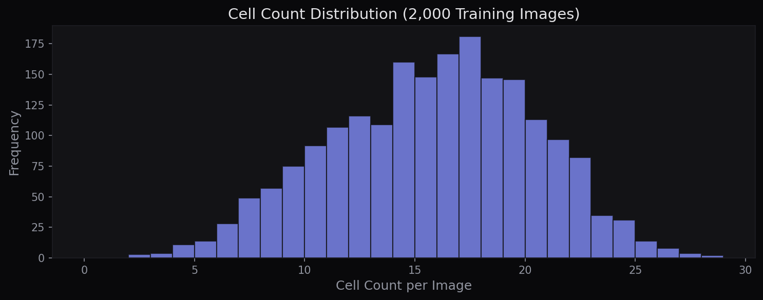
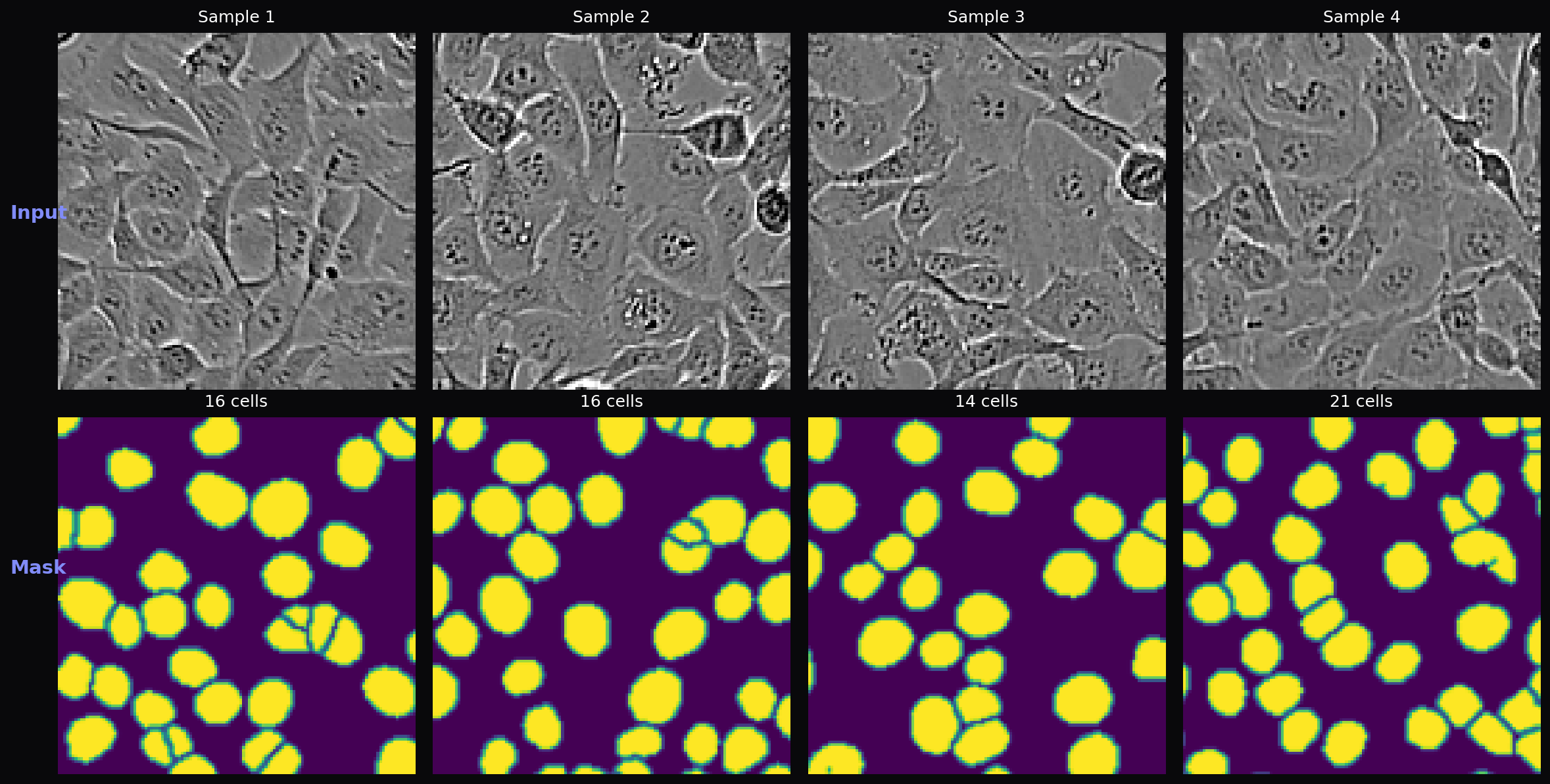
The dataset contains 2,000 grayscale fluorescence microscopy images (128×128 pixels) with binary cell masks. Cell counts per image range from 2 to 28 (mean 15.3). An additional 2,000 unlabeled test images are used for Kaggle evaluation. Following the original U-Net paper’s emphasis on augmentation for biomedical images, the training pipeline applies elastic deformation, random flips, 90° rotations, Gaussian noise, and brightness/contrast adjustment.
Frameworks & Tools
How It Works
Encoder (Contracting Path): Four downsampling blocks progressively extract features at increasing spatial abstraction. Each block applies two 3×3 convolutions with BatchNorm and ReLU, then MaxPool2d to halve the spatial dimensions. Feature channels double at each level: 64 → 128 → 256 → 512, with a 1024-channel bottleneck. This captures both fine-grained cell boundaries and global context about cell distribution.
Decoder (Expanding Path): Four upsampling blocks use transposed convolutions to recover spatial resolution. At each level, the upsampled features are concatenated with the corresponding encoder features via skip connections, preserving fine spatial detail lost during downsampling. The Attention U-Net variant adds attention gates before each concatenation, learning a spatial attention mask that highlights cell regions and suppresses background noise.
Cell Counting: The model outputs a single-channel probability map, which is binarized at threshold 0.5. Morphological opening removes small noise blobs, closing fills holes within cells, and binary hole-filling handles any remaining gaps. SciPy’s connected-component labeling then assigns a unique ID to each contiguous cell region. Components smaller than 10 pixels are filtered as noise. For touching cells, an optional watershed step uses the distance transform to find cell centers and separate overlapping regions.
Challenges & Solutions
- Touching cells merged into one — Adjacent cells with overlapping boundaries were counted as a single cell. Addressed with morphological post-processing and watershed-based separation using distance transforms to identify individual cell centers
- Class imbalance (background >> cells) — Cell pixels constitute a small fraction of each image, causing BCE loss to converge on “predict all background.” Solved with the combined BCE+Dice loss, where Dice directly optimizes the overlap metric regardless of class proportions
- Overfitting on 2,000 images — The ~31M parameter U-Net easily overfits with limited training data. Mitigated with aggressive data augmentation (especially elastic deformation, which the original U-Net paper identifies as critical for biomedical images), ReduceLROnPlateau scheduling, and best-model checkpointing
- No proper input normalization initially — Early versions fed raw [0, 255] pixel values through the network without normalization, causing unstable gradients. Fixed by normalizing to [0, 1] in the dataset class, which immediately improved convergence
References
- Ronneberger, O. et al. (2015). “U-Net: Convolutional Networks for Biomedical Image Segmentation.” MICCAI. arXiv:1505.04597
- Oktay, O. et al. (2018). “Attention U-Net: Learning Where to Look for the Pancreas.” MIDL. arXiv:1804.03999